Project Report | League of Legends Match Prediction Using Laning Phase Data
[Project-Report Machine-Learning Data-Analysis Game-Analytics Author: Jinhang Jiang
Master of Science in Business Analytics at Arizona State University, Class 2021
Introduction
League of Legends is a team-based strategy game where two teams of five powerful champions face off to destroy the other’s base.(Source)
A typical League of Legends game tends to last 30 to 45 mins, and each game can be divided into three phases: the laning phase, mid game, and late game. Players normally spend the first 10 to 15 minutes to farm in their own lanes (Top, Mid, Bot, JG) to gain early advantages in builds and levels. In the middle game phase, players start to focus on the macro level: push lanes, take down towers, get map objectives, and group fights. In the late game, if the game has not ended, each team has to decide how to close the game, for examples: force a baron/elder dragon or 1–4 push, etc.
In this project, I used the data collected by the Kaggle named “michel’s fanboi,” and the dataset contains the first 10min. stats of approx. 10k ranked games (SOLO QUEUE) from a high ELO (DIAMOND I to MASTER). You may find the full description and data source here.
The champion combos of each team will significantly impact the results of the games since some champions are strong in the early game, while other champions will be scaling greatly throughout the mid and late game. And that is why all the rank games and professional games will have a ban/pick phase prior to the games. However, a lot of influences that players can make to the game with their skills and map awareness will not be reflected by the champion combos. Especially, some players, like RNG.Uzi, can gain significant advantages in the laning phase regardless of if the opponents have counter-picks or not.
Also, as we can see, in a lot of high-level games, team combos, especially the combos for the late game, did not always work out as expected since the laning phase tends to have more uncertainties than the mid and late game phases, such as one of the teams was able to create a gap that was too big for the other team to fill up in the late game. My goal is to understand how the laning phase performance (the first 10 mins) affects the final result.
I used the Jupyter Notebook and R studio as the code editors. I did some data exploration with Pandas, NumPy, and Matplotlib packages. Then, I implemented nine models, including an ensemble model, a stacking model, and seven other classifiers. The most consistent model was the stacking model, whose average accuracy score on cross-validation was 0.732158, with a standard deviation of +/- 0.005171.
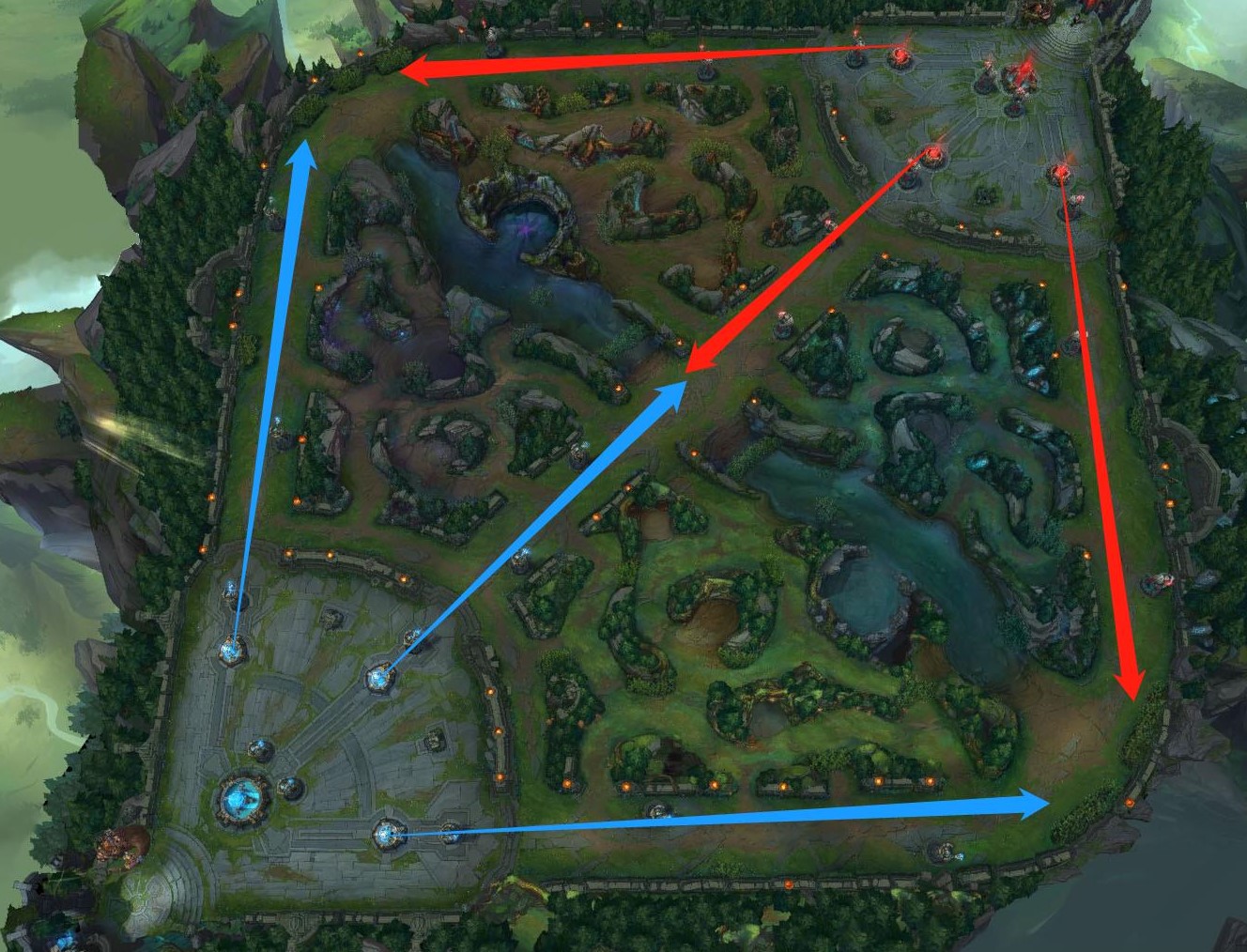
League of Legends: Blue Team (Left) vs. Red Team (Right)
Data Explore
The dataset has the information of 9879 games in total, and the blue teams won 4930 of them, which is 49.9%. It is a very balanced dataset.
Figure 1 shows the number of kills by both teams. Purple points were for the red-team wins, and yellow points meant the blue teams won the games. I learned that the blue teams won all the games when they had more than 15 kills in the first 10 mins. The winning rate for the blue teams started to increase after getting 7 kills dramatically.
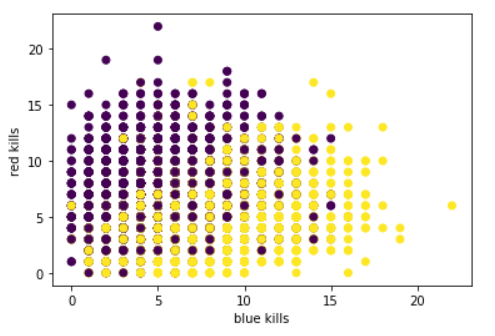
Figure 1: Blue vs. Red in Kills
Figure 2 shows the number of assists by both teams. It had the same pattern with the kills plot. However, there is only one game for each team to get more than 20 kills in the laning phase, while there are many games that both teams were able to get more than 20 assists in the laning phase. It suggested that most kills could have come from the bottom lane or the junglers ganked a lot.
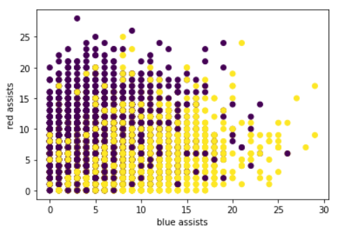
Figure 2: Blue vs. Red in Assists
Figure 3 shows the comparison in gold. This plot gave me an obvious indication that if the blue teams could get more than 20,000 gold in the first 10 minutes, they were extremely likely to win the games. I also manually set a “green zone,” which covered the games in which the blue teams were able to get more than 21,055 gold in the first 10 minutes. The blue teams won all the games that fell in the “green zone” in this data sample.
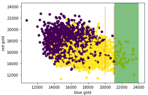
Figure 3: Blue vs. Red in Gold
Then, I studied the relationship between the gold difference the blue teams made in the laning phases and the games’ results. Figure 4 shows that when the blue teams have a gold difference between -6324 and 6744 in the first 10 mins (the red zone), the games were very flippable, and the final results could favor either side.
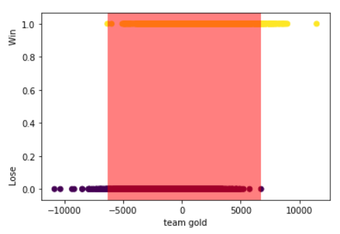
Figure 4: Gold Difference for Blue Team by W/L
In the games of League of Legends, it would be easier for the teams with better vision in the mid and late game to gain initiatives. Yet, how important the vision was in the early game? Figure 5 does not indicate any importance of vision in the early games, which was somewhat beyond my expectations.
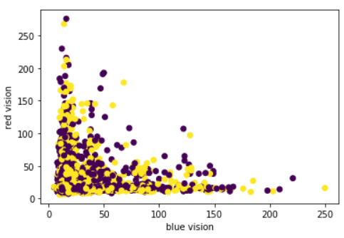
Figure 5: Blue vs. Red in Vision
Figure 6 illustrates the relationship between the experience difference that the blue team had in the laning phase and the results of the games. The games were really 50–50 when the experience difference was roughly +/- 5000 XP in the first 10 minutes. In a normal framing game, the mid laners and top laners can reach level 8, and the bot laners and junglers can reach level 6, respectively, at roughly 10 minutes. It takes 1150 XP from level 7 to level 8, and it takes 880 XP from level 5 to level 6. A 5000 XP advantage means approximately 1 level higher on average (1150*2+880*3=4940) for every lane in the early games.
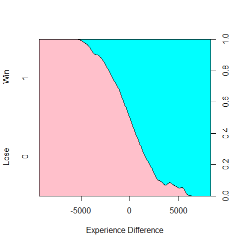
Figure 6: Experience Difference for Blue Team by W/L
Apart from the above, there are some fun statistics I want to share:
- When the blue teams’ KDA was larger or queal to 3 in the first 10 minutes, they had a 76.51% winning rate.
- When the blue teams could destroy a tower in the first 10 minutes, they had a 75.43% winning rate.
- When the blue teams were able to have 8 kills in the first 10 minutes, they had a 69.86% winning rate.
Feature Engineering
Since there are many features with large values, such as Experience, Total Gold, etc. I applied the StandardScaler() and the MinMaxScaler() to those features. After testing, I decided to use StandardScaler() transformation for the rest of the project.
I also created the following features:
blueKDA/redKDA: The kill to death ratio for the blue teams in the first 10 minutes. It was calculated by [(blueKills+blueAssists)/blueDeaths]. I used the same procedure to create redKDA as well.
KDADiff: The KDA difference between the two teams. It was calculated as (blueKDA-redKDA).
blueGoldAdv: This feature is a binary variable. It indicates if the blue teams had at least a 20,000 gold advantage in the games’ first 10 minutes.
blueDiffNeg: This feature is a binary variable. It indicates if the blue teams had a negative gold difference less than or equal to -6324 in the first 10 minutes of the games.
blueDiffPos: This feature is a binary variable. It indicates if the blue teams had a positive gold difference more than or equal to 6744 in the first 10 minutes of the games.
Modeling
Because I did not really have a holdout set to test my models’ effectiveness, I chose to use the cross-validation technique and use accuracy and ROC as the evaluation metrics.
I tested the following nine models:
AdaBoostClassifier, CatBoostClassifier, XGBoostClassifier,
Support Vector Classifier, LogisticRegression, RandomForestClassifier,
KNeighborsClassifier,EnsembleVoteClassifier, StackingClassifier
eclf = EnsembleVoteClassifier(clfs=[cat,logreg, knn, svc,ada,rdf,xgb], weights=[1,1,1,1,1,1,1])
    labels = ['CatBoost','Logistic Regression', 'KNN', 'SVC','AdaBoost',"Random Forest",'XGBoost','Ensemble']
    cv=KFold(n_splits = 5, random_state=2022,shuffle=True)
    for clf, label in zip([cat,logreg, knn, svc, ada, rdf, xgb,eclf], labels):
        scores = cross_val_score(clf, info_x, info_y,
                                cv=cv,
                                scoring='accuracy',
                                n_jobs=-1)
        print("[%s] Accuracy: %0.6f (+/- %0.6f) Best: %0.6f "
            % (label,scores.mean(), scores.std(), scores.max()))
Figure 7 shows the outputs of the nine models. After hyperparameters tuning, the stacking model had an average accuracy of 0.732158, the third-best score. Still, it also had the lowest standard deviation, indicating that it did the best job of preventing overfitting in the cross-validation test. The ensemble model and stacking model also had the best and second-best ROC score. This outcome was consistent with what I discussed in the previous post: Simple Weighted Average Ensemble | Machine Learning.
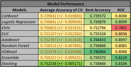
Figure 7: Model Performance Table
Figure 8 is the ROC plots for all the models that I mentioned above:
plt.figure()
    lw = 1
    #knn
    knn.fit(X_train,y_train)
    knn_pred = knn.predict_proba(X_test)
    fpr, tpr, threshold = roc_curve(y_test,knn_pred[:,1])
    roc_auc = auc(fpr, tpr)
    plt.plot(fpr, tpr, color='tab:blue',
         lw=lw, label='KNN ROC curve (area = %0.4f)' % roc_auc)
    ... ...
    ... ...
    ... ...

    plt.plot([0, 1], [0, 1], color='navy', lw=lw, linestyle='--')
    plt.xlim([-0.02, 1.0])
    plt.ylim([0.0, 1.05])
    plt.xlabel('False Positive Rate')
    plt.ylabel('True Positive Rate')
    plt.title('ROC curve')
    plt.legend(loc="lower right")
    plt.show()
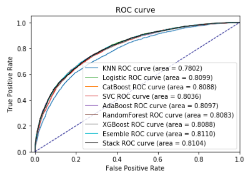
Figure 8: ROC Plots on Testing Dataset
False Prediction Analysis
At the end of this project, I split the dataset into training and testing datasets with a ratio of 7 to 3 and fitted the training dataset with the stacking model. Then, I did a little more analysis specifically on the instances that my model wrongly predicted. I wanted to understand that under what kind of conditions the games would become more unpredictable.
Figure 9 and Figure 10 illustrate the total gold and total experience of the two teams in the first 10 minutes. Those two plots clearly show that teams with the early advantages in gold and experience ended up losing the game. There were 799 wrong predictions in the test set.
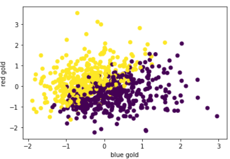
Figure 9: Blue vs. Red in Gold for the Wrong Predictions
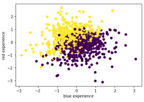
Figure 10: Blue vs. Red in Experience for the Wrong Predictions
I also took a step further to look at the performance of the junglers since, in the laning game, both teams’ laners usually need help from junglers to gain initiatives. Figure 11 shows the junglers’ performance. This is the average difference between “blueTotalJungleMinionsKilled” and “redTotalJungleMinionsKilled” for the whole testing dataset, wrong predictions, and correct predictions, respectively. The “JGDiff” for the wrong predictions is smaller than the average level of the whole testing dataset, which means when the blue junglers outperformed the average, the prediction will become a little bit harder.

Figure 11: Junglers Performance Difference
Conclusion
My models clearly hit a bottleneck since none of them could produce an accuracy score higher than 0.75. My assumption is that the final dataset only contains 44 features, a very low-dimensional dataset given that League of Legends could potentially catch hundreds of variables from each game. For further experiments, I would recommend incorporating features, like the champion combos, time frames, champion proficiency for specific players, etc. into the analysis.
League of Legends has been one of the most popular games globally in the past decade. It brought the players from different continents together and let them share pleasures in the Summoner’s Rift. Even though I tried to predict the outcomes of the ranking games, I have always had the understanding that the only way to keep the game fascinating is to make it as unpredictable as possible. The most exciting moments are always for the ultimate group fights following by the big comebacks. The famous jungler, RNG.MLXG, once said, “if you don’t know how to flip a losing game, why to bother playing League of Legends.”
You may find the code of this project in my GitHub repository.
